Working with SOFA files

The Quick tour of SOFA and sofar showed how to access SOFA files. In many cases you will want to have a closer look at the data inside a SOFA file or use it for further processing. In this section, you will see examples of how to do that using pyfar.

Retrieving data for specific source and receiver positions

In most cases SOFA files contain data for lots of source or receiver positions and it is often important to get data for a specific position. An elegant way of doing that is to use pyfar Coordinates and Audio objects. Coordinate objects have built in methods to search specific positions and they can convert between a large variety of coordinate systems for you. For audio objects, there is a growing pool of functions for plotting and processing that comes in handy. If you installed sofar, pyfar was installed as a part of it.

You have two options to get SOFA data into pyfar. The first option is to load the SOFA file with sofar.read_sofa and then manually generate Audio and Coordinates objects from the data inside the SOFA file. The second option is to use pyfar.read_sofa, which directly returns the Audio and Coordinates objects. Let’s be lazy and do that. For more information on pyfar checkout the examples that are part of the pyfar documentation.

import pyfar as pf
import numpy as np
import os
import matplotlib as mpl
import matplotlib.pyplot as plt

# select matplotlib backend for plotting
%matplotlib inline

# load head-related impulse responses
hrirs, source_coordinates, receiver_coordinates = pf.io.read_sofa(
    os.path.join('data', 'head_related_impulse_responses.sofa'))

Matplotlib is building the font cache; this may take a moment.

The SOFA file used in this example contains head-realated impulse responses (HRIRs) from the FABIAN database. Let’s find the HRIR for the source position at the left ear on the horizontal plane. It has an azimuth angle of 90 degrees and an elevation of 0 degrees.

# coordinate point to find
find = pf.Coordinates().from_spherical_elevation(np.pi/2, 0, 1.7)
# index of corresponding point
lateral, _ = source_coordinates.find_nearest(find, k=1)

print(lateral)

(134,)

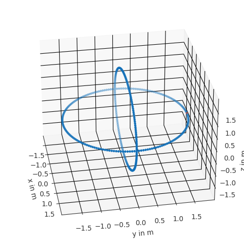
This tells us that the HRIR for the desired source position is at index 134 in the hrirs audio object. Note that you get more then the closest point by using larger values for k. We can use the Coordinates.show method to get visual feedback for checking if we got the correct source

source_coordinates.show(lateral)
plt.gca().view_init(azim=-10)

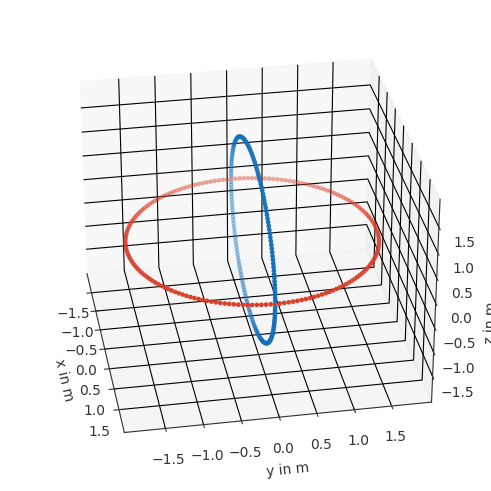
Let’s also find all sources on the horizontal plane, i.e., all sources that have an elevation of 0 degree. Let’s get visual feedback right away. This time, we don’t get an index but a logical array with True at the positions where source_coordinates.elevation is zero.

horizontal = source_coordinates.elevation == 0
source_coordinates.show(horizontal)
plt.gca().view_init(azim=-10)

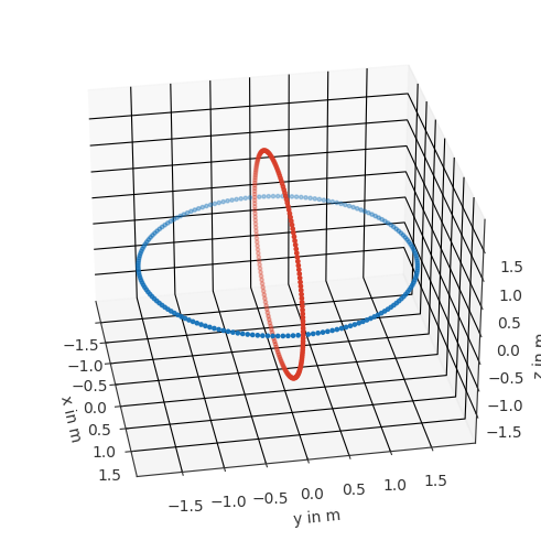
For completeness, let’s also find all sources in the median plane. This can be done in a similar way, considering that they have a lateral angle of 0 degree

median = source_coordinates.lateral == 0
source_coordinates.show(median)
plt.gca().view_init(azim=-10)

Plotting

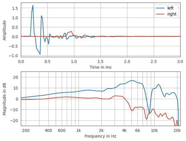
Plotting data is a very common task and can be easy with the help of the pyfar plot module. Let’s start with plotting the HRIR (time signal) and HRTF (magnitude response) for the lateral source position.

ax = pf.plot.time_freq(hrirs[lateral], unit='ms', label=['left', 'right'])
ax[0].set_xlim(0, 3)
ax[0].legend()
ax[1].set_ylim(-25, 25)

(-25.0, 25.0)

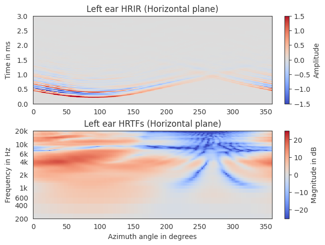
Plotting the entire horizontal plane is also easy, however, a few more lines are required for a nicer formatting

azimuth = np.round(source_coordinates.azimuth[horizontal] / np.pi * 180)

ax, qm, cb = pf.plot.time_freq_2d(
    hrirs[horizontal, 0], indices=azimuth, unit='ms',
    cmap=mpl.colormaps['coolwarm'])

ax[0].set_title("Left ear HRIR (Horizontal plane)")
ax[0].set_xlabel("")
ax[0].set_ylim(0, 3)
qm[0].set_clim(-1.5, 1.5)

ax[1].set_title("Left ear HRTFs (Horizontal plane)")
ax[1].set_xlabel("Azimuth angle in degrees")
ax[1].set_ylim(200, 20e3)
qm[1].set_clim(-25, 25)

The median plane HRIRs could be plotted in a similar way.

Processing

For detailed information about sofar refer to the sofar documentation. Pyfar also offers methods for digital signal processing we won’t detail all of them, but let’s at least look at a few common tasks. For everything else, check out the pyfar documentation.

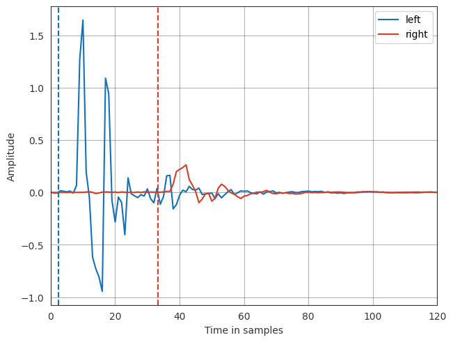
Find HRIR onset

Finding the onset or starting point of an HRIR is a common task, for example to compute the interaural time difference or to time align HRIRs for further processing. A common way of finding the onset is to detect the first sample in the HRIR that is less than 20 dB below the absolute maximum value. Let’s find this point for our lateral HRIR

# low-pass HRIR at 3 kHz
hrir_onset = pf.dsp.filter.butterworth(hrirs[lateral], 10, 3000)
# upsample by a factor of 10 for subsample accuracy
hrir_onset = pf.dsp.resample(hrir_onset, 10 * hrirs.sampling_rate)
# find the onset
onset = pf.dsp.find_impulse_response_start(hrir_onset, 20) / 10
# the low-pass introduces a low frequency group-delay of 15 samples, which we
# need to correct. you can see the group delay in a simple plot if running:
# lp = pf.dsp.filter.butterworth(pf.signals.impulse(2048), 10, 3000)
# pf.plot.group_delay(lp, unit='samples')
onset -= 15

# plot the result
ax = pf.plot.time(hrirs[lateral], unit='samples', label=['left', 'right'])
ax.axvline(onset[0], color=pf.plot.color('b'), linestyle='--')
ax.axvline(onset[1], color=pf.plot.color('r'), linestyle='--')
ax.set_xlim(0, 120)
ax.legend()

<matplotlib.legend.Legend at 0x7fd479e7beb0>

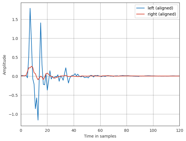
Align HRIRs

Aligning HRIRs is often done as a pre-processing step before HRIR interpolation. Now that we already estimated the onsets, aligning the HRIRs can be done by means of a cyclic fractional time shift

hrirs_aligned = pf.dsp.fractional_time_shift(
    hrirs[lateral], -onset, mode='cyclic')

ax = pf.plot.time(hrirs_aligned, unit='samples',
                  label=['left (aligned)', 'right (aligned)'])
ax.set_xlim(0, 120)
ax.legend()

<matplotlib.legend.Legend at 0x7fd479ed2f80>

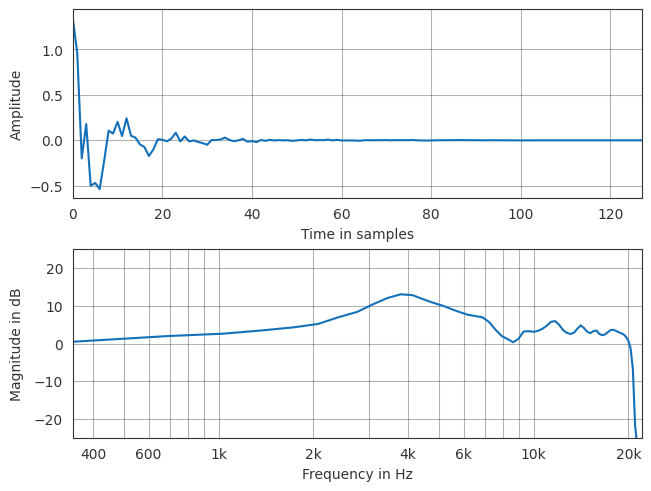
Compute diffuse-field HRIR

The diffuse field HRIR can be obtained by averaging across source positions. This is a common task and also easy if using pyfar

# obtain energetic average using equal weights. Unequal weights can be realized
# using the `weights` parameter.
diffuse_field_hrir = pf.dsp.average(hrirs, mode='power')

# obtain minimum phase version, since the energetic averaging resulted in zero-
# phase HRIRs
diffuse_field_hrir = pf.dsp.minimum_phase(diffuse_field_hrir)

# plot
ax = pf.plot.time_freq(diffuse_field_hrir, unit='samples')
ax[1].set_ylim(-25, 25)

(-25.0, 25.0)

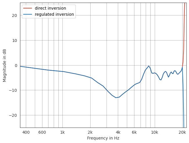
Generate headphone compensation filter

If using HRIRs for binaural synthesis, i.e., spatial audio playback, we need a headphone compensation filter. A good and easy approximation is to use the inverted diffuse field HRIR. We can see from the plot above that the diffuse field HRIR does not contain energy above 20 kHz. A direct inversion would thous not be good. We use a regulated inversion instead.

direct_inversion = 1 / diffuse_field_hrir
regulated_inversion = pf.dsp.regularized_spectrum_inversion(
    diffuse_field_hrir, [0, 20_000])

ax = pf.plot.freq(direct_inversion, color='r', label='direct inversion')
pf.plot.freq(regulated_inversion, color='b', label='regulated inversion')
ax.set_ylim(-25, 25)
ax.legend()

<matplotlib.legend.Legend at 0x7fd479d7d150>