
Working with SOFA files#
The Quick tour of SOFA and sofar showed how to access SOFA files. In many cases you will want to have a closer look at the data inside a SOFA file or use it for further processing. In this section, you will see examples of how to do that using pyfar.
Retrieving data for specific source and receiver positions#
In most cases SOFA files contain data for lots of source or receiver positions and it is often important to get data for a specific position. An elegant way of doing that is to use pyfar Coordinates and Audio objects. Coordinate objects have built in methods to search specific positions and they can convert between a large variety of coordinate systems for you. For audio objects, there is a growing pool of functions for plotting and processing that comes in handy. To use pyfar install it into you python environment
$ pip install pyfar
You have to options to get SOFA data into pyfar. The first option is to load
the SOFA file with sofar.read_sofa and then manually generate Audio
and Coordinates objects from the data inside the SOFA file. The second option
is to use pyfar.read_sofa, which directly returns the Audio and
Coordinates objects. Lets be lazy and do that
import pyfar as pf
import matplotlib as mpl
import matplotlib.pyplot as plt

data_ir, source_coordinates, receiver_coordinates = pf.io.read_sofa(
    'FABIAN_HRIR_measured_HATO_0.sofa')
The SOFA file used in this example is contained head-realated impulse responses (HRIRs) from the FABIAN database. Lets find the HRIR for the source position at the left ear on the horizontal plane. It has an azimuth angle of 90 degrees and an elevation of 0 degrees
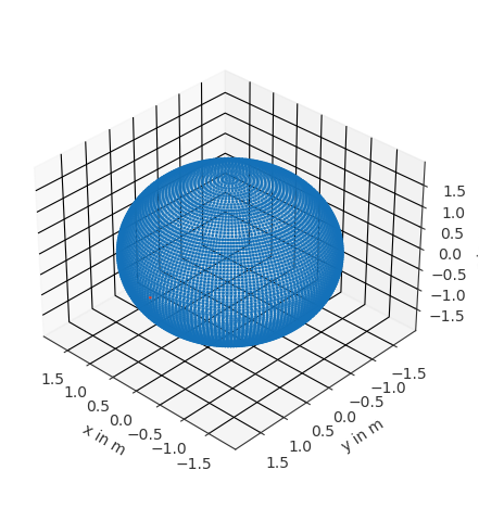
index, *_ = source_coordinates.find_nearest_k(
    90, 0, 1.5, k=1, domain='sph', convention='top_elev', unit='deg', show=True)
The variable index = 5930 tells us where to find data for the desired
source position. Since we used show=True we also get visual feedback for
checking if we got the correct source
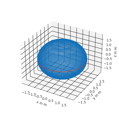
Note that you get more then the most closest point by using different values
for k. It is also possible to all source positions on or in the vicintiy
of the horizontal plane using the find_slice method of the Coordinates
object. Sources on the horizontal plane have zero degree elevation and thus can
be obtained by
_, mask = source_coordinates.find_slice(
    'elevation', unit='deg', value=0, show=True)
Again, we get visual feedback if we want
Plotting data#
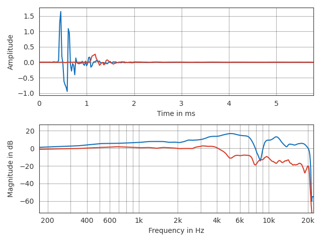
Ploting can be done with the built in plot functions. For example to take a look at the time data and magnitude spectra of a single source position
pf.plot.time_freq(data_ir[index])
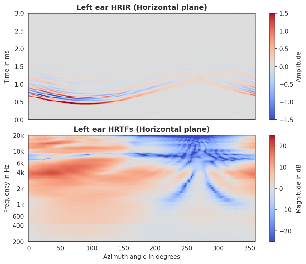
Plotting the entire horizontal plane is also a one liner using
pf.plot.time_freq_2d, however, a few more lines are required for a nicer
formatting
with pf.plot.context():

    plt.subplots(2, 1, figsize=(8, 6), sharex=True)

    angles = source_coordinates.get_sph('top_elev', 'deg')[mask, 0]

    ax, qm, cb = pf.plot.time_freq_2d(data_ir[mask, 0], indices=angles,
                                    cmap=mpl.cm.get_cmap(name='coolwarm'))

    ax[0].set_title("Left ear HRIR (Horizontal plane)")
    ax[0].set_xlabel("")
    ax[0].set_ylim(0, 3)
    qm[0].set_clim(-1.5, 1.5)

    ax[1].set_title("Left ear HRTFs (Horizontal plane)")
    ax[1].set_xlabel("Azimuth angle in degrees")
    ax[1].set_ylim(200, 20e3)
    qm[1].set_clim(-25, 25)

    plt.tight_layout
Next steps#
For detailed information about sofar refer to the SOFA objects and sofar functions documentation. Pyfar also offers methods for digital signal processing that wont be detailed here. A god way to dive into that is the pyfar documentation and the pyfar examples notebook.